
Select the analytical function to transform to s-domain.
Used for damped functions e^(at) sin(ωt) as ω.
Numeric evaluation point for F(s).
A Laplace transform calculator helps you convert a time-domain function into its corresponding s-domain expression. It is widely used in calculus, differential equations, electrical engineering, control systems, and signal processing.
Our Laplace Transform Calculator is designed to help you work with common functions such as powers of time, exponential functions, sine, cosine, and damped oscillations. Enter the function and its required parameters to calculate the transform and, where supported, evaluate the result at a selected value of s.
The calculator can help you check homework, verify mathematical expressions, and understand how Laplace transforms simplify differential equations. You can also use the formulas and worked examples below to follow the calculation step by step.
About Laplace Transform Calculator
This Laplace transform calculator converts a time-domain function f(t) into its s-domain form F(s). It also shows the region of convergence (ROC), and it can evaluate F(s) at a specific value of s.
It is built for students in differential equations, circuits, signals and systems, or control courses. It also suits engineers checking a hand calculation. Before you start, know your function, the constants in it (such as the exponent n, the decay rate a, or the angular frequency ω), and whether you want a number at a particular s or the full expression.
Table of Contents
How to Use the Laplace Transform Calculator
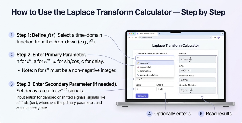
Follow these steps to calculate the Laplace transform of a supported time-domain function.
- Choose the time-domain function: Select the function that matches your expression, such as a power of t, exponential, sine, cosine, or damped oscillation.
- Enter the primary parameter: Depending on the selected function, enter the required value for n, a, ω, or c.
- Enter the secondary parameter: Some damped or shifted functions require an additional value. Enter it when the calculator requests it.
- Enter a value of s (optional): If you want to evaluate the transformed expression at a particular point, enter the required s value.
- Click Calculate: The calculator will display the mathematical result and relevant properties supported by the selected function.
- Review the result: Check the transformed expression and its region of convergence before using the result in another calculation.
A few details are important when entering parameters:
- The angular frequency ω is measured in radians per second, not hertz.
- For a signal with frequency f in hertz, convert it using ω = 2πf.
- The sign of the exponential parameter matters. For example, e⁻²ᵗ represents a decaying exponential.
- Trigonometric functions use radians.
Always check the selected function and parameter values before calculating.
Understanding the Results
A Laplace transform changes a time-domain function f(t) into an s-domain function F(s). This makes many calculus operations easier to handle algebraically.
The main results and terms you should understand include:
- F(s): The transformed function expressed in terms of the complex variable s.
- Time-domain function f(t): The original function defined over time.
- Region of Convergence (ROC): The set of values of s for which the Laplace transform integral converges.
- Evaluated F(s): A numerical result obtained by substituting a selected value of s into the transformed expression, provided that the value is inside the ROC.
- Transformation operator: The notation ℒ{f(t)} = F(s), which represents the relationship between the original function and its transform.
The region of convergence is an important part of the result. For example, the transform of e²ᵗ is 1/(s − 2), but its ROC is Re(s) > 2. Substituting a value outside this region may produce an algebraic number, but that number does not represent a convergent Laplace transform integral.
The Laplace Transform Formula
The one-sided Laplace transform, also called the unilateral Laplace transform, is defined by:
[F(s)=\mathcal{L}{f(t)}=\int_0^\infty e^{-st}f(t),dt]
Where:
- f(t) = the original time-domain function
- t = time
- s = a complex frequency variable
- F(s) = the Laplace transform of f(t)
- e⁻ˢᵗ = the exponential kernel used in the transformation
The complex variable s is commonly written as:
[s=\sigma+j\omega]
Here, σ represents the real part and ω represents the imaginary-frequency component.
The Laplace transform is useful because it converts differential equations into algebraic equations in the s-domain. After solving the algebraic equation, the inverse Laplace transform can be used to recover the time-domain solution.
The one-sided transform starts at t = 0. It is therefore commonly used for initial-value problems where the initial conditions are known.
Laplace Transform Table
A Laplace transform table contains standard transform pairs that help you identify the transformed form of common functions without evaluating the integral every time.
The following table includes frequently used one-sided Laplace transforms.
| Time-domain function f(t) | Laplace transform F(s) | Region of convergence | ||
|---|---|---|---|---|
| 1 | 1/s | Re(s) > 0 | ||
| t | 1/s² | Re(s) > 0 | ||
| tⁿ, n = 0, 1, 2, … | n!/sⁿ⁺¹ | Re(s) > 0 | ||
| eᵃᵗ | 1/(s − a) | Re(s) > a | ||
| t eᵃᵗ | 1/(s − a)² | Re(s) > a | ||
| sin(ωt) | ω/(s² + ω²) | Re(s) > 0 | ||
| cos(ωt) | s/(s² + ω²) | Re(s) > 0 | ||
| sinh(at) | a/(s² − a²) | Re(s) > | a | |
| cosh(at) | s/(s² − a²) | Re(s) > | a | |
| e⁻ᵃᵗ sin(ωt) | ω/((s + a)² + ω²) | Re(s) > −a | ||
| e⁻ᵃᵗ cos(ωt) | (s + a)/((s + a)² + ω²) | Re(s) > −a | ||
| u(t − c), c ≥ 0 | e⁻ᶜˢ/s | Re(s) > 0 |
Here, u(t − c) represents the unit step function, and n is a non-negative integer in the power-function formula.
Important Properties of Laplace Transforms
You can use a few important properties to calculate more complicated transforms from standard transform pairs.
1. Linearity
[\mathcal{L}{\alpha f(t)+\beta g(t)}
=\alpha F(s)+\beta G(s)]
This means you can transform each part of a sum separately and then combine the results.
2. Frequency Shifting
[\mathcal{L}{e^{at}f(t)}=F(s-a)]
Multiplying a time-domain function by an exponential shifts its transform along the s-domain.
3. Time Shifting
[\mathcal{L}{f(t-c)u(t-c)}=e^{-cs}F(s)]
This property is useful for functions that begin after a delay.
4. Derivative Properties
[\mathcal{L}{f'(t)}=sF(s)-f(0)]
[\mathcal{L}{f”(t)}=s^2F(s)-sf(0)-f'(0)]
These derivative rules are especially important when solving differential equations because they introduce the initial conditions directly into the s-domain equation.
Worked Example: Damped Sine Wave
Consider the function:
[f(t)=e^{-2t}\sin(3t)]
We want to find its Laplace transform and evaluate it at s = 1.
The standard formula for a damped sine function is:
[\mathcal{L}{e^{-at}\sin(\omega t)}
=\frac{\omega}{(s+a)^2+\omega^2}]
For this example:
- a = 2
- ω = 3
- s = 1
Substitute the values:
[F(s)=\frac{3}{(s+2)^2+3^2}]
Simplify:
[F(s)=\frac{3}{(s+2)^2+9}]
Expanding the denominator:
[F(s)=\frac{3}{s^2+4s+13}]
Now evaluate at s = 1:
[F(1)=\frac{3}{(1+2)^2+9}]
[F(1)=\frac{3}{18}=\frac{1}{6}\approx0.1667]
The region of convergence is:
[\operatorname{Re}(s)>-2]
Since s = 1 satisfies this condition, the evaluation is valid.
Worked Example: Inverse Laplace Transform
The inverse Laplace transform converts an s-domain expression back into its time-domain function. It is commonly used after solving a differential equation in the s-domain.
Consider:
[F(s)=\frac{1}{(s+1)(s+3)}]
First, use partial fractions:
[\frac{1}{(s+1)(s+3)}
=\frac{A}{s+1}+\frac{B}{s+3}]
Solving for A and B gives:
[A=\frac{1}{2},\qquad B=-\frac{1}{2}]
Therefore:
[F(s)=\frac{1}{2}\frac{1}{s+1}
-\frac{1}{2}\frac{1}{s+3}]
Using the standard inverse transform pairs:
[\mathcal{L}^{-1}\left{\frac{1}{s+a}\right}=e^{-at}]
The time-domain result is:
[f(t)=\frac{1}{2}(e^{-t}-e^{-3t}),\quad t\geq0]
This example shows how partial fractions make inverse Laplace calculations easier.
Piecewise Functions
A piecewise function uses different expressions over different time intervals. Laplace transforms can handle these functions by representing them with unit step functions.
For example, consider a function that equals 2 from t = 0 to t = 3 and becomes zero afterward:
[f(t)=
\begin{cases}
2,&0\leq t<3\
0,&t\geq3
\end{cases}]
It can be written using unit step functions:
[f(t)=2u(t)-2u(t-3)]
Using the standard Laplace transform and time-shifting property:
[F(s)=\frac{2}{s}-\frac{2e^{-3s}}{s}]
Therefore:
[F(s)=\frac{2(1-e^{-3s})}{s}]
Because this function is nonzero only over a finite time interval, its Laplace integral converges for every finite complex value of s.
Piecewise functions are common in engineering applications involving switching signals, delayed inputs, and systems that change behavior over time.
The Laplace Transform of y in Differential Equations
Laplace transforms are particularly useful when solving differential equations with known initial conditions.
Suppose you have the differential equation:
[y’+2y=0]
with the initial condition:
[y(0)=5]
Let Y(s) represent the Laplace transform of y(t).
Using the derivative property:
[sY(s)-5+2Y(s)=0]
Collect the terms:
[(s+2)Y(s)=5]
Therefore:
[Y(s)=\frac{5}{s+2}]
Taking the inverse Laplace transform gives:
[y(t)=5e^{-2t}]
This approach changes a differential equation into an algebraic equation that is easier to solve. It is especially helpful for linear differential equations with initial conditions.
Common Situations Where the Calculator Helps
The Laplace transform calculator can be useful in several mathematical and engineering applications.
- Homework and exam preparation: Check transform formulas and verify solutions to practice problems.
- Differential equations: Convert differential equations into algebraic equations in the s-domain.
- Electrical circuits: Analyze RC, RL, and RLC circuit responses.
- Control systems: Work with transfer functions, system responses, and stability analysis.
- Signal processing: Study time-domain signals and their corresponding s-domain expressions.
- Engineering calculations: Verify standard transform pairs and parameter substitutions.
The calculator is a useful way to check supported expressions, while the formulas and examples help you understand the mathematical steps.
Common Mistakes
Laplace transform calculations can become confusing when parameters, signs, or convergence conditions are handled incorrectly.
- Ignoring the ROC: A transformed expression is not the complete answer without its region of convergence. Check that the selected s value lies inside the ROC before evaluating it.
- Mixing up exponential signs: The transforms of eᵃᵗ and e⁻ᵃᵗ have different denominator shifts and convergence conditions.
- Using hertz instead of radians per second: Convert frequency using ω = 2πf before entering it into a sine or cosine function.
- Forgetting initial conditions: The transform of a derivative includes the function’s initial value. Do not simplify it to sF(s) unless the relevant initial condition is zero.
- Using the wrong power formula: For non-negative integer n, the transform of tⁿ is n!/sⁿ⁺¹. For non-integer powers, the gamma function may be required.
- Applying inverse transforms incorrectly: Check the partial fraction decomposition and match each term with the correct inverse transform pair.
- Ignoring the one-sided assumption: The unilateral transform describes the function from t = 0 onward. It does not automatically represent behavior before time zero.
Checking these details can help you avoid common algebraic and mathematical errors.
Laplace Transform vs. Fourier Transform
Laplace and Fourier transforms are related mathematical tools, but they are used for different purposes.
| Feature | Laplace Transform | Fourier Transform |
|---|---|---|
| Main purpose | Analyze systems, differential equations, and growth or decay | Analyze frequency content |
| Variable | Complex variable s | Frequency variable |
| Exponential behavior | Can handle growing and decaying exponential functions within its ROC | Requires suitable convergence conditions |
| Initial conditions | Commonly used in initial-value problems | Not directly incorporated in the same way |
| Applications | Control systems, circuit analysis, differential equations | Signal processing, frequency analysis, communications |
The Fourier transform can be viewed as the Laplace transform evaluated along the imaginary axis, provided that the imaginary axis lies inside the region of convergence.
Use the Laplace transform when you need to study system behavior, initial conditions, or exponential growth and decay. Use the Fourier transform when your main goal is to understand a signal’s frequency components.
Accuracy, Assumptions, and Limitations
The calculator is designed around standard Laplace transform definitions and supported function families. However, the results depend on selecting the correct function and entering its parameters accurately.
Keep these points in mind:
- One-sided transform: The standard formula used here starts at t = 0 and does not calculate a bilateral Laplace transform.
- Supported functions: The calculator may not support every possible mathematical expression. More complicated functions can require manual rewriting.
- Region of convergence: An evaluated result is meaningful only when the selected s value lies inside the ROC.
- Parameter accuracy: Incorrect signs, frequency units, or parameter values can change the transformed expression.
- Numerical precision: Decimal evaluations may be rounded for display. Use the exact symbolic expression when further algebraic work is required.
- Inverse calculations: Inverse Laplace transforms require a supported s-domain expression input. Do not assume this feature is available unless it is implemented in the calculator interface.
For advanced mathematical or engineering work, verify important results using the defining integral, a trusted transform table, or an independent symbolic mathematics tool.
Practical Tips
- Check the ROC first: Make sure your selected value of s satisfies the convergence condition before evaluating F(s).
- Convert frequency correctly: If the input frequency is given in hertz, convert it to angular frequency in radians per second.
- Check exponential signs: Pay attention to whether the function contains eᵃᵗ or e⁻ᵃᵗ.
- Use standard transform pairs: A transform table can help you identify the correct formula quickly.
- Include initial conditions: When transforming derivatives, include the required initial values.
- Verify your algebra: Expand denominators and check partial fraction decompositions before accepting a result.
- Understand the output: Do not rely only on the numerical evaluation. Review the symbolic expression and ROC to understand the complete result.
Frequently Asked Questions
What is the Laplace transform of 1?
The Laplace transform of the constant function 1 is:
[\mathcal{L}{1}=\frac{1}{s}]
Its region of convergence is Re(s) > 0.
What is the Laplace transform of eᵃᵗ?
The Laplace transform of an exponential function is:
[\mathcal{L}{e^{at}}=\frac{1}{s-a}]
Its region of convergence is Re(s) > a.
Can a Laplace transform calculator solve differential equations?
A Laplace transform calculator can help calculate Laplace transforms used when solving differential equations. Solving a complete differential equation may also require applying initial conditions, rearranging the s-domain equation, and finding an inverse transform.
What is the region of convergence?
The region of convergence is the set of values of s for which the Laplace transform integral converges. It is an essential part of the transform because the same algebraic expression can represent different time-domain functions under different convergence conditions.
Why does my evaluated value look incorrect?
Check that your selected s value lies inside the region of convergence. Also verify the sign of the exponential parameter and make sure angular frequency is entered in radians per second rather than hertz.
Is the Laplace transform of a derivative simply sF(s)?
Not always. For the first derivative, the correct formula is:
[\mathcal{L}{f'(t)}=sF(s)-f(0)]
It becomes sF(s) only when the initial value f(0) is zero.
What is the difference between Laplace and inverse Laplace transforms?
The Laplace transform converts a time-domain function f(t) into an s-domain expression F(s). The inverse Laplace transform converts F(s) back into its corresponding time-domain function, subject to the relevant assumptions and convergence conditions.
Why are Laplace transforms used in electrical engineering?
They help engineers analyze circuit responses, transfer functions, and system behavior. They also simplify differential equations involving capacitors, inductors, and other circuit components.
Can I use a Laplace transform table instead of calculating the integral?
Yes. A transform table provides standard pairs that can be used to identify common transforms quickly. You can also combine table entries with properties such as linearity, frequency shifting, and time shifting.
Calculate Laplace Transforms More Easily
Laplace transforms provide a practical way to simplify differential equations and analyze time-dependent systems. They are widely used in mathematics, electrical engineering, signal processing, and control systems.
Use the calculator above to work with supported time-domain functions, review the transformed expressions, and evaluate F(s) when appropriate. Combine the results with the transform table, formulas, and worked examples on this page to understand each step and verify your calculations.
For arithmetic that comes up around the same coursework, you can use our Percentage Calculator, Average Calculator, and GPA Calculator. More tools in this area are on the Math Calculators page.